Understanding machine learning #3: Confusion matrix – not all errors are equal

One of the most typical tasks in machine learning is classification tasks. It may seem that evaluating the effectiveness of such a model is easy. Let’s assume that we have a model which, based on historical data, calculates if a client will pay back credit obligations. We evaluate 100 bank customers and our model correctly guesses in 93 instances. That may appear to be a good result – but is it really? Should we consider a model with 93% accuracy as adequate?

It depends. Today, we will show you a better way to evaluate prediction models.

Not all errors are equal

Let’s come back to our example. The model was only wrong in 7 instances, however, its true quality depends on which instances. Let’s say that out of 100 clients, only 10 would not pay back. In this case, we can assume two scenarios:

• Out of 7 errors, 6 will be a situation in which the person would pay back but was assumed not to pay and one instance is the reverse
• Out of 7 errors, 6 will be a situation in which the person wouldn’t pay back but was assumed to pay and one instance is the reverse

Obviously, the second scenario is more costly to the bank, which suffered significant loss because it gave loans to people who didn’t manage to repay. To better explain this whole process, let’s introduce these terms:

• Positives – are instances that have the value we are looking for when using a prediction model. Usually, they are less common values: for example, clients that actually buy our insurance or a client who will not pay back his loan.
• Negatives – are instances that are more popular in the sample. For example, healthy people (when we are looking for sick ones) or clients who actually will buy our product (when we try to phone them).

True and false negatives

Indeed, there are two categories of error: predicting a positive when the instance is negative and predicting a negative when the instance is positive. There are also two categories of good prediction; successful prediction is called true and unsuccessful false. As you can see, we now have 4 variants which form a tighter confusion matrix.

Let’s get back to our example. We have 100 loan clients.

Out of the 100, 10 will not pay back their loan (positives). However:

1. We correctly identified 8. So in 8/10 instances we prevented loss [TRUE POSITIVES]
2. We incorrectly identified 2. So in 2/10 instances we didn’t prevent loss [FALSE NEGATIVES]

The other 90 people paid back their loans (negatives). However:

1. We correctly identified 85. So in 85/90 we gave a loan to people who paid us back [TRUE NEGATIVES]
2. We incorrectly identified 5. So in 5/90 we didn’t give a loan to people who would pay us back. A loss but smaller than in the previous case. [FALSE POSITIVES]

Confusion matrix

This information in a table will form the confusion matrix.

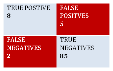
When we sum it up (8+2+85+5), we get all of our 100 clients.

This method of evaluation is more meaningful, so let’s look next at a model taking into account spcific goals.